Problem statement – CVRP with Traffic Jams

On this page, you can find a condensed report on a study of Dynamic Capacitated Vehicle Routing with Traffic Jams (CVRPwTJ). This variant is our proposal of adding dynamic elements into the classical and well-studied CVRP, which in turn is an extension of VRP. All of the problems fall into combinatorial optimization and integer programming.

The relationship between the problems is as follows:

VRP – there is an undirected and complete graph of N locations (N-1 customers and the depot) and a fleet of m vehicles. Each edge connecting two locations has a traverse cost (Euclidean distance). The goal is to visit each customer exactly once by a vehicle while minimizing the total cost of the routes. Each route must originate and terminate in the depot.

CVRP – in addition to VRP, each customer has a certain demand of goods. The vehicles have identical capacities, that denote how many of the goods they can serve. Because each customer must be served exactly once, the maximum amount of demand cannot exceed the vehicles’ capacity.

CVRPwTJ – in addition to CVRP, the cost of traversing an edge in the locations graph is affected by traffic conditions. The conditions may change during the realization of the problem according to certain probability distributions, which makes it dynamic and stochastic in contrast to VRP and CVRP.

The evaluation procedure

Unlike in static optimization problems such as VRP and DCVRP, the final result depends on the traffic situation, which is unknown until it actually happens. Therefore, the solution is constructed dynamically during a simulation. We will refer to this simulation as “the main simulation” to distinguish it from o Monte Carlo simulations aimed at testing various actions/modifications without applying them to the actual solution yet. Apart from the impact (constructing the actual solution vs. testing possible scenarios), both types of simulations have the same structure.

The simulations are divided into discrete time steps.

In each step:

• The current traffic situation is calculated.
• At least one vehicle must be assigned a non-empty visiting schedule. We will call such vehicles active. Here, the MCTS/UCT approach is employed to calculate this schedule.
• Active vehicles are moved from the current locations to the next ones according the their schedules. This is performed as an atomic operation regardless of how long the distances are.
• The total cost of the simulation is incremented by the sum of edges traversed by the vehicles.
• Unless the problem is solved (i.e. all vehicles returned to the depot and all clients are served), the simulation proceeds to the next step.

How a traffic situation is calculated:

We introduce three variables controlling the traffic simulation:

For each edge, P stands for the probability that a TJ will be imposed on it in the current time step. If TJ is imposed on the edge a, its regular cost c(a) is multiplied by a random intensity I(a) for the timespan of L(a) steps.

We have tested the following values of P: 0.02, 0.05 and 0.15. I(a) and L(a) were selected from uniform random distributions U_{_INT}[10,20] and U_{_INT}[2,5], respectively.

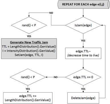
Figure: How the traffic conditions in the simulation are applied.

We assume that although benchmark problems include exact realizations of TJ computed by certain probability distributions, any method used for solving the CVRPwTJ problem has access only those distributions. The actual realizations of the traffic jams are visible to the method only after they happen. Therefore, a method may use the fact that the global probability P = 0.05 (for example) and what range the intensities and lengths can be in, but not when or where the TJ will be imposed.

The main idea of the proposed approach

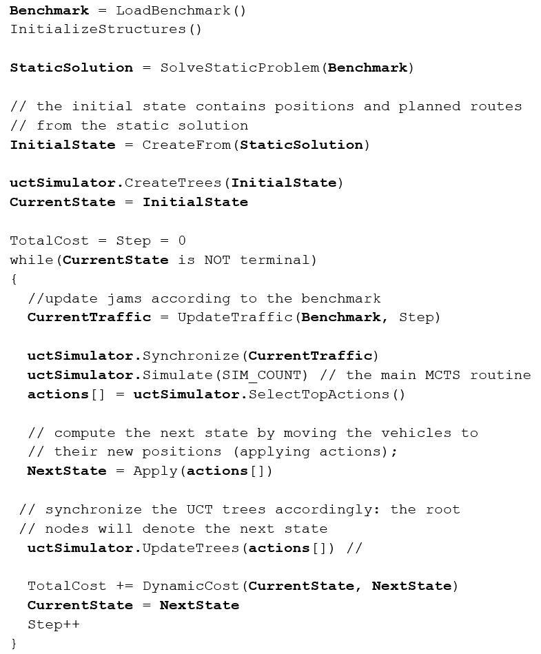
In short, our idea of solving the problem with use of MCTS/UCT is based on the following steps:

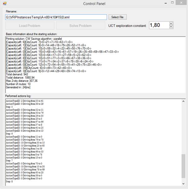
• We decided to start from the initial solution – computed for the static version of the problem – rather than using MCTS to solve the problem from scratch, because the latter approach was completely infeasible due to the combinatorial complexity of the problem. The initial solution of choice is the Clark and Wrights savings algorithm.
• For each route present in the initial solution, a UCT tree is created. At the beginning, the trees are in simply paths with the first and the last elements being a depot. The consecutive elements on each path denote the clients visited by respective trucks in subsequent time steps. For example, the fourth elements in all paths represent the set of clients visited in the third step of the solution.
• A top-down overview of the method can be found here.
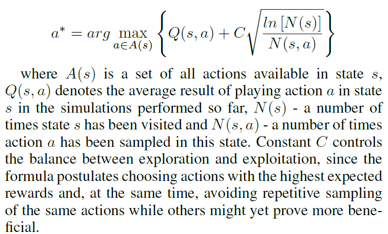
• The internal UCT simulations are performed simultaneously in all UCT trees. At each time step, and action is chosen in each tree. The next compound step (movement of all k trucks) is a result of a combined knowledge obtained from all trees.
• An action in a tree represents moving the truck according to the schedule or changing the schedule (in order to test a different one). In order to limit the state-space search, we defined various types of sensible actions which can be used by the MCTS/UCT algorithm.
• All proposed actions are based on the following underlying rationale: if the currently selected candidate edge is not jammed then traverse it, otherwise try to enhance the
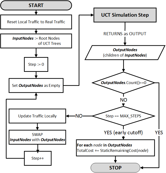
  planned route (by avoiding the traffic jam) by means of local changes in the planned orders of visited clients. We have defined actions, which modify on 0, 1 or 2 existing routes, respectively.
• A simulation ends when there are no more active trees (all trucks have completed their routes) or the step counter reaches a pre-defined threshold value of MAX STEPS (the so-called Early Termination), whichever comes first. We set MAX STEPS to be equal to the maximum length of a traffic jam
• Once the simulation is completed, the sum of traversed costs from all k trees is back-propagated from the last visited nodes in each tree to the root nodes. When the Early Termination condition is applied, the sum of static costs (i.e. without TJ consideration) computed for the remaining fragments of the routes is added to the score

Benchmarks and Results

We have used some of the known benchmark instances available for CVRP and injected the information about the traffic jams. The file format used for this study is specified in this text document. You can download the base versions, i.e. without the traffic jams, here [9 KB]. Next you can use the tool provided below to insert traffic jams into the downloaded files.

Convertion-generation tool [Download] [17 KB]

Using this tool you can load a file, which is either a third-party CVRP file (three formats are supported) or the CVRP file in our format either with or without the traffic jams inside. When working with the former case, clicking the Convert button will generate the file compliant with our CVRPwTJ problem. Such a generated file may be loaded again using the Select file and then injected with the traffic jams using the Generate button. If any traffic data is already contained it will be overwritten.

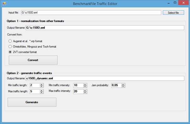
The injection of the traffic jams is performed based on the probability distributions discussed earlier. For each out of 10 tested benchmarks, we used the same intensity and length distributions and three options for probability values: 0.02, 0.05, 0.15 for light, medium and heavy traffic, respectively. That counts as 30 distinct benchmark instances. For each instance, we generated 50 test cases with various probability realizations, what gives 1500 tests in total.

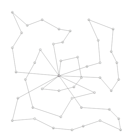
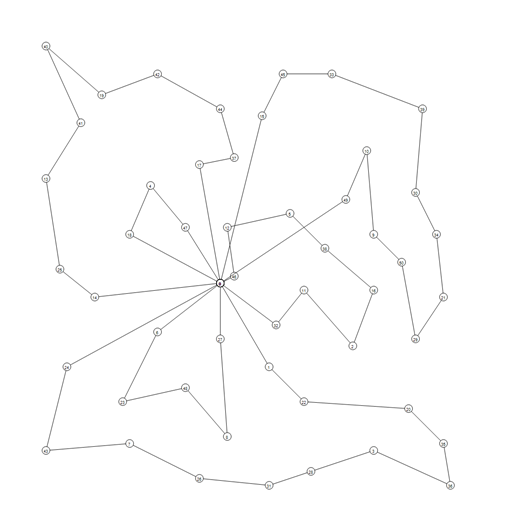
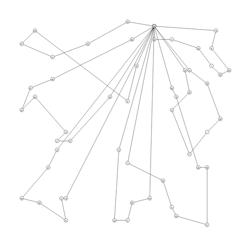
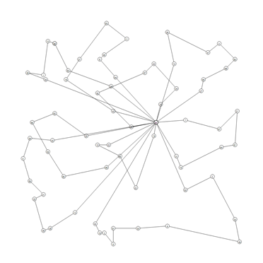
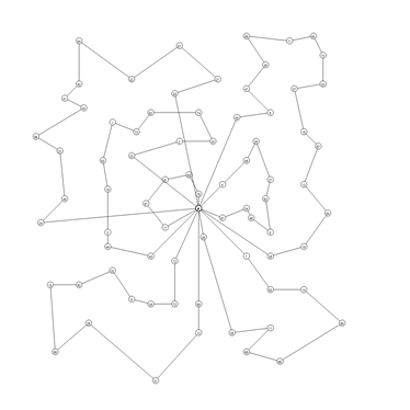
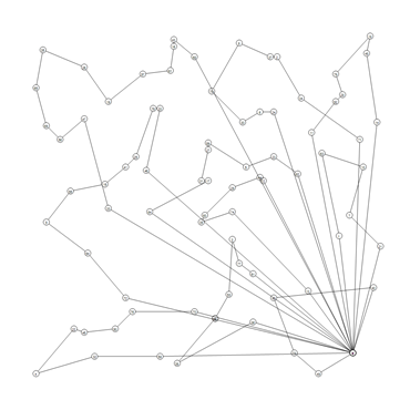
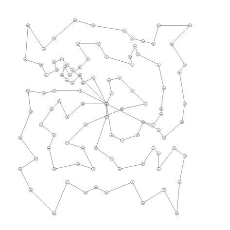
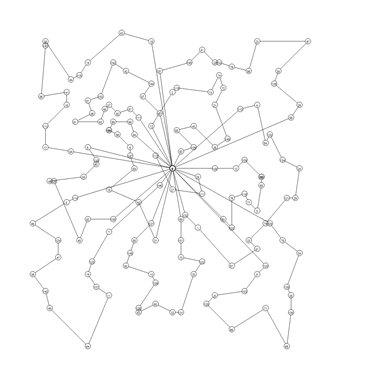
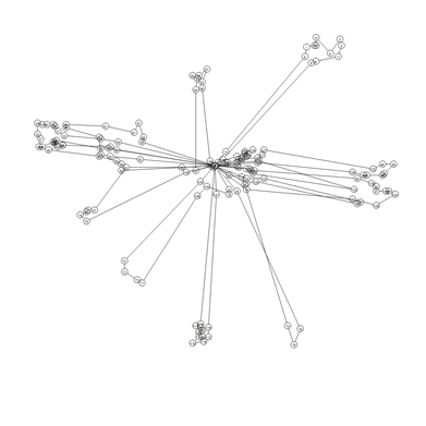
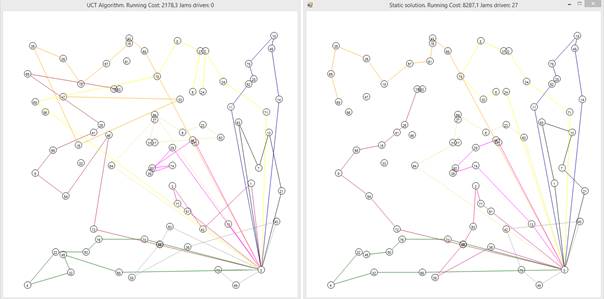
Below, we present the used benchmark with sample graphical results of the solutions:

Benchmark Name	Visual representation
P-n19-k2
P-n45-k5
E-n51-k5
A-n54-k7
A-n69-k9
E-n76-k5
A-n80-k10
P-n101-k4
C-n150D-k5
Tai-n150b-k5