Resource-Constrained Project Scheduling Problem (RCPSP)
The Resource-Constrained Project Scheduling Problem (RCPSP) is one of relatively popular NP-complete optimization problems. Each deterministic single-mode RCPSP instance defines a number of activities as well as renewable resources and their capacities.
All activities must be performed for the project to be finished. Each of them requires a certain amount of time and resources – it cannot be started unless sufficient amounts of resources of each required type are available. Additionally, activities may have predecessors, i.e. activities that must be performed before their successor may be started. Typically, activities are not preemptive – once started they cannot be stopped until they are finished, which effectively means that it is illegal to split one activity into several smaller ones.
RCPSP’s goal is finding a legal schedule that minimizes the makespan of the project.
Risk-Aware Project Scheduling Problem (RAPSP)
While RCPSP is one the problems that are especially interesting due to their almost direct applicability to real-life scenarios, it does still introduce a significant level of simplification that may actually hinder its usefulness in at least some cases.
Therefore, we have defined a new class of problems, namely Risk Aware Project Scheduling Problems (RAPSP). This new model introduces, in addition to standard elements of RCPSP, non-determinism of activity durations, external risks that may influence the project and risk responses that may be undertaken by the project team, e.g. to mitigate or avoid some of the risks. We feel that especially this last addition makes the problem interesting, and for multiple reasons. Firstly, inclusion of risk management processes makes the problem even closer to actual real-life scenarios. Secondly, the dynamic characteristics of the task make it an especially good testbed for various AI- and CI-based approaches.
RAPSP, building on top of RCPSP, adds several new concepts:
- non-deterministic activity durations taking into account unavoidable mistakes in estimations
- non-renewable resources – as in multi-mode RCPSP
- risks – unpredictable external events that may influence the project characteristics and definition in various ways
- risk responses – special activities that do not have to be completed but have effects influencing project parameters (analogically to risks)
RAPSP activities’ durations are not defined as constant values like in RCPSP, but rather as random variables with known probability distributions.
Risks model unpredictable external events that may influence the project. While each risk may be different, they are always defined by their realization conditions, occurrence probabilities and effects.
Risk responses represent various actions that may be taken by the Project Manager to manage or handle project risks. These would typically be aimed at either reducing the probability of risk occurrence or mitigating its effects. Risk responses may, however, be performed both reactively and proactively, and their effects will take place whether or not any risks have occurred. Risk responses are, in this sense, totally independent of risks themselves.
Risk responses are defined as special kinds of activities that do not have to be performed (in general) for the project to be successfully finished. Just like any activity, risk responses may have positive duration and may require resources. Once a risk response is finished, its effect will occur and influence the project characteristics.
It should be noted that, due to non-deterministic nature of RAPSP, it is impossible to solve it by simply generating a schedule for the realization of the project. Instead, it is necessary to make a series of decisions, choosing activities and risk responses to perform depending on current conditions and random variables realizations. In other words, a strategy needs to be devised. RAPSP solvers represent such strategies.
RAPSP Solvers
Heuristic Solver (HS)
Heuristic Solver (HS) is based on a popular and relatively simple RCPSP solver, which employs a prioritization rule and Parallel Schedule Generation Scheme (PSGS) to generate a schedule. In each time step, it starts legal activities in the order defined by the prioritization rule. Only when there are no more eligible activities does the algorithm move to the next time step.
Employing this approach in RAPSP obviously requires some modifications. Basically HS realizes the project by devising a baseline schedule, trying to follow it as long as the deviation from it is not too big and regenerating it in case of major deviations, i.e. in decision points.
Finally, in each decision point we need to come up with a new baseline schedule. To achieve that, our Heuristic Solver (HS) starts by creating a number of randomly chosen legal combinations of risk responses that can be started immediately and a priority rule. For each such combination a simulation is performed. It starts with execution of the selected risk responses. Afterwards, the project is converted to a simplified deterministic version, by replacing all activity duration values with expected values of their distributions and removal of non-realized risks. A schedule for this deterministic project is than generated according to PSGS with the selected priority rule. This schedule, together with its subset of risk responses, becomes a baseline schedule candidate. The candidate with the shortest makespan is then selected as the baseline schedule to be used for the RAPSP project till the next decision point.
GRASP
GRASP stands for Greedy Randomized Adaptive Search Procedure and is an iterative process for solving combinatorial problems, which we apply to solving Stochastic Resource-Constrained Project Scheduling subproblem of RAPSP.
The overall process is similar to the one employed by the HS algorithm. In each decision point, each legal combination of possible risk responses is tried (or a random subset of those combinations if their number exceeds a predefined threshold). For each such combination GRASP algorithm is used to generate a candidate strategy for a non-deterministic project with no further risk responses. Expected makespans of projects realized according to those strategies are calculated as a side product and this allows to easily choose the best risk responses–strategy combination. This combined strategy is followed till the next decision point.
BasicUCT
UCT stands for Upper Confidence bounds applied to Trees and is a simulation-based method of solving problems based on tree representation. While it is nowadays known mainly for its popularity in the domain of game-playing, most notably Go, it can actually be quite successful also in other problem areas. In practice, it can act as a decision-maker for many finite Markov processes, or problems that can be expected to remain relatively similar to them – such as RAPSP.
Proactive UCT (ProUCT)
Proactive UCT (ProUCT) is a more sophisticated solver that combines the mostly reactive behavior of HS or GRASP with proactive capabilities of UCT-based approach. During the UCT simulations only two kinds of actions are available: starting a legal risk response or letting the HS / GRASP algorithm follow its own policy for a number of time units. As soon as a decision point is reached (or a predefined maximum number of time units passes) control is transferred back to the UCT algorithm. In other words, a single UCT action encompasses the whole process of using HS / GRASP algorithm for several time units.
Experiments
Problem Instances
Obviously, there exists no standard set of RAPSP problem instances. Therefore, we decided to generate our test projects by modifying RCPSP instances provided by the standard and popular PSPLIB Library. To that extent we have developed a procedure for transforming RCPSP samples into RAPSP instances.
Firstly, it would replace activity duration values with random variables with known distributions – thus converting RCPSP into SRCPSP. Additionally, 10% of the activities with the highest duration values would be selected as resource-intensive. These would be modified so that each of them would require 1 unit of a dedicated non-renewable resource. Exactly 1 unit of each resource would also be added to the project.
Second transformation phase involved adding risks and risk responses. A single risk was added for each resource type whose effect would be a temporary or permanent (depending on configuration) decrease in the capacity of this resource by 1 or 2 units. A corresponding risk response would require a number of time units and a certain amount of a dedicated non-renewable resource (budget) to temporarily or permanently increase the amount of the resource by 1 unit. Finally, the transformation would add serious underestimation risks and corresponding risk responses of performing activities with capital-intensive approach.
In order to test the solvers for projects of varying characteristics we introduced 3 transformation modes:
- Temporary Effects with Separate Budgets (TSep): In this mode non-renewable resource risks and risk responses would have temporary effects. This meant that no combination of risks and risk responses could render the project a failure by making it impossible to finish all activities. Each of the three categories of risk responses would also require its own kind of dedicated budget non-renewable resource.
- Temporary Effects with Shared Budget (TSh): TSh differed from TSep in that only one type of budget was introduced and required by all risk responses.
- Permanent Effects with Separate Budgets (PSep): In this mode risk response budgets were again separate, but non-renewable resource risk and risk-response effects were permanent. This meant that certain combinations of risks could lead to a project failure and this threat could be multiplied by poor risk response budget management.
Results
We tested the solvers on several thousand problem instances in total. Highly non-deterministic nature of the task introduced obvious need for a higher number of tests to reach meaningful results. To make the comparison as fair as possible each tested problem instance would always be solved by each and every algorithm. Additionally, to minimize the randomness of the results we would set up our random number generators so as to minimize differences within each set of tests, i.e. should all the solvers make the same decisions for a given problem instance, they would all yield the same result (because same risks would occur at the same time). However, since mid-project decisions may influence risk occurrence conditions, this does not necessarily mean that exactly the same risks would always occur for each solver, so some level of ambiguity of comparison would always remain.
We performed the experiments on projects with 30, 60 and 120 activities, using, respectively, 480, 480 and 100 problem instances for each project size and transformation mode (therefore doing 3180 test runs in total).
We calculated two statistics: average relative project duration and win rate. Since project makespans could differ significantly and we had no way of finding meaningful minimal makespan values for our projects, for each problem instance we measured the solvers results in relation to the best makespan achieved. That meant that for each project at least one method would be assigned a result of 100%, and the others would be proportionally higher. The latter statistic (win rate) was simply the number of experiments in which given solver achieved the best result (relative project duration of 100%) in relation to the total number of experiments. Since multiple solver could achieve the same result for any given problem instance, win rates did not have to sum up to 100%.
TSep
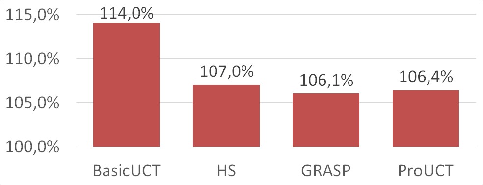
TSep: relative project durations
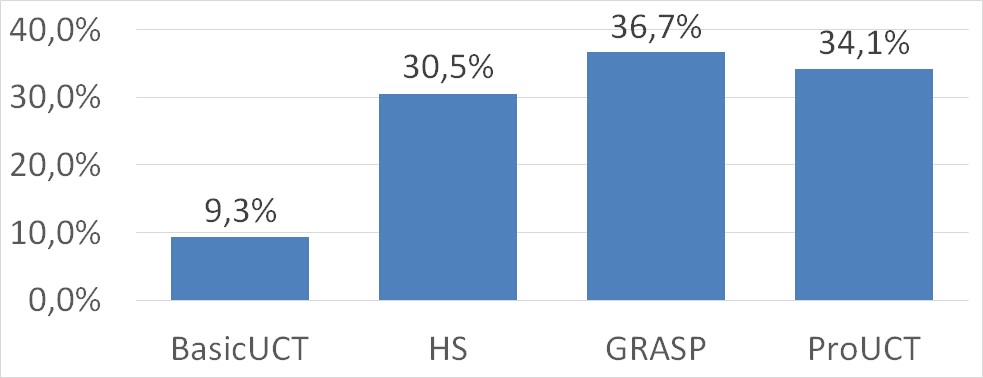
TSep: solvers win rates
As expected, BasicUCT fared significantly worse than all other methods, and ProUCT achieved slightly (but statistically significantly) better results than HS. GRASP solver was even more successful – its advantage over ProUCT was, however, statistically not significant.
Tsh
TSh experiment involved one shared non-renewable resource acting as a risk-response budget. This added more complexity to the problem, as more risk-management strategies were possible and more risk response related decisions could be made. In other words: problem search space was visibly widened.
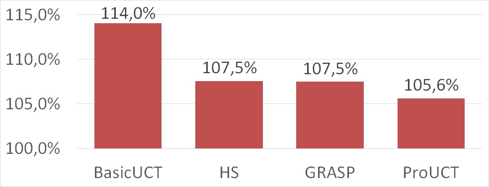
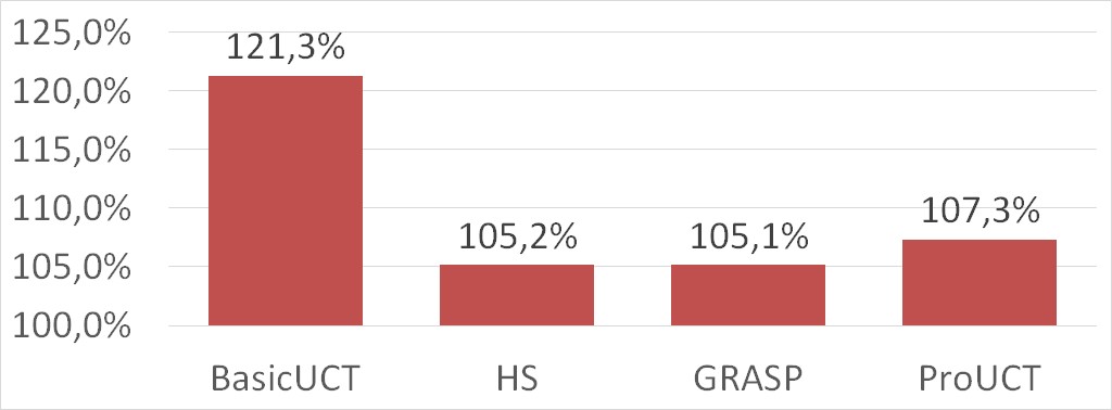
TSh: relative project durations
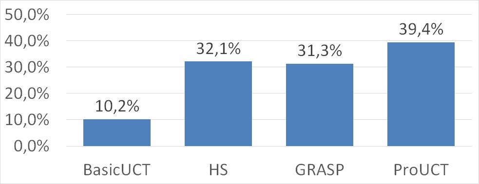
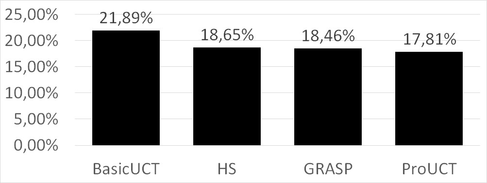
TSh: solvers win rates
This change had a clear impact on the solvers performance. This time HS and GRASP solver performed almost exactly on par, and ProUCT achieved a definite victory over both of. This can be explained by the proactive nature of the ProUCT algorithm and it being definitely best-suited for dealing with risk responses via the use of UCT algorithm. GRASP’s and HS’es simplified handling of risk responses turned out to be a significant burden.
PSep
PSep problem instances introduced one crucial change: those projects could fail, i.e. reach a state in which it was impossible to finish the project due to lacking non-renewable resources. Dealing with this kind of risk requires more careful risk-management strategies and not using risk response budgets too early.
PSep: relative project durations

PSep: solvers win rates
PSep: solvers failure rates
To analyze the results of this experiment we also needed to slightly redefine statistics for measuring performance of the solvers. Firstly, when calculating average relative project duration for each solver, we would consider only successful projects. Secondly, we would calculate another statistic: failure rate, measuring the ratio of failed projects for each algorithm.
Results are interesting. BasicUCT remains, as always, the poorest possible algorithm choice. While differences between HS and GRASP remain not very significant, ProUCT’s results beg for some further analysis. While its average relative duration is higher and win rate lower than its competition, it, at the same time, has the lowest failure rate. This can be explained by high penalty for project failure, which biased the UCT algorithm towards safer strategies, instead of trying to aggressively reduce the expected makespan of the project. This kind of approach can be expected to be, in most cases, preferable in real-life projects.